Bayesian Data Analysis: Fitting a Curve to Data

I recently went back to some notes I wrote for a lecture on Bayesian statistics for first year astronomy graduate students. I think Bayesian statistics can be pretty straightforward in terms of the logic used to solve problems, however, the computational methods can be complicated. In the literature when we see Bayesian methods in use we often see specialized, computationally expensive ones like Markov chain Monte Carlo (MCMC) and Nested Sampling. When it comes to multi-dimensional analyses or those with non-trivial correlation, these methods are often necessary. For simpler 1D or 2D problems we can use similiarly simpler methods that better illustrate the underlying machinery of Bayesian data anlsyis.

One of the most fundamental problems of data anlaysis is fitting a line to data. We usually pose this problem as an example of parameter estimation: we wish to estimate the slope of the line and the uncertainty of our estimate. We may also be interested in whether a line is the prefered model for the data: why not a quadratic, some other polynomial, or some other curve altogether? The Bayesian framework naturally gives us a way to perform model selection in addition to parameter estimation.

In this Python example we will consider two models (or hypotheses) for position v. time data: (\(\mathcal{H}_v\)) constant velocity motion, (\(\mathcal{H}_a\)) constant acceleration motion. We will determine the best fit line and quadratic for our data, calculating the Bayesian evidence for each. Then we compare evidence to determine which model better fits the data.

The concepts of marginalization, likelihoods, priors, Bayesian evidence, Bayes factors, and odds ratios were covered in the lecture. If you’ve never heard of those before, you’ll have trouble following along. I also use probability notation that I introduced in the lecture, and I’m not going to explain it here.

Fitting Curves to Data

Lets get started by loading some standard Python libraries.

import numpy as np
import matplotlib.pyplot as plt
import scipy.integrate

Given some position v. time data, and we want to know if the object was moving at constant velocity or accelerating.

constant velocity:

\[x(t) = x_0 + v_0 t\]

constant accleration:

\[x(t) = x_0 + v_0 t + \frac{1}{2} a_0 t^2\]

simulate data

We start by defining a function to compute the position of the particle as a function of the initial position, velocity, and acceleration.

def pos_v_time(t, x0=0, v0=0, a0=0):
    """position of object undergoing constant acceleration"""
    ts = np.asarray(t)
    xs = x0 + v0*ts + 0.5*a0*ts**2
    return xs

Now we pick the initial conditions for our simulated data. We’ll start the object at \(x_0 = 0\). We will simulate a slowly accelerating object, to make it harder to tell the difference between constant velocity and acceleration. Lets choose \(v_0 = 24\) cm/s and \(a_0 = 6\) cm/s\(^2\).

We need to add in some simulated measurement error to the position v. time data. Lets say our position measuring instrument has uncertainty at the 4 cm level.

T = 3.0  # length of data (sec)
dx = 4  # cm of meas uncert
x0 = 0
v0 = 24  # cm/s
a0 = 6  # cm/s^2

ts = np.arange(0, T, 0.2)
xs = pos_v_time(ts, x0, v0, a0)
N = len(ts)

uncert = np.random.normal(scale=dx, size=N)

x_dat = xs + uncert
x_dat[0] = 0  # x=0 defined!

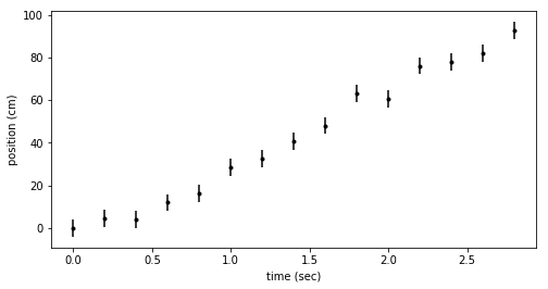
Here’s a plot of the simulated data. As we intended, it’s hard to tell if the particle is accelerating or not. Are these data better fit with a line or a quadratic?

fig = plt.figure(figsize=(8,4))
ax = fig.add_subplot(111)
ax.errorbar(ts, x_dat, yerr=dx, fmt=".k")
ax.set_xlabel('time (sec)')
ax.set_ylabel('position (cm)')

constant velocity (linear) model

Now we’ll calculate the evidence for the constant velocity model. In general this model depends on \(x_0\) and \(v\). For our data we said \(x_0 = 0\) by definition, so there is one free parameter, \(v\).

The evidence is the marginal likelihood for the model. We must marginalize the likelihood over all of the free parameters, in this case just \(v\):

\[p\left(d \mid \mathcal{H}_v \right) = \int \mathrm{d}v \, p\left(v \mid \mathcal{H}_v \right)\, p\left( d \mid \mathcal{H}_v, v \right)\]

This will give us the probability for the constant velocity model averaged over all possible \(v\)’s rather than for a specific choice of one. The integral has two terms: the likelihood as a function of \(v\) and the prior probability for \(v\).

We’ll use a Gaussian likelihood, which compares our model \(m\) to the data \(d\). Each data point has the same \(\sigma = 4\) cm.

\begin{align*} m_i = x_i &= v\, t_i, \\
p\left(d \mid \mathcal{H}_v, v \right) &= \left(\frac{1}{\sqrt{2\pi}\,\sigma}\right)^N \exp\left(- \frac{(d_i-m_i)^2}{2{\sigma}^2}\right) \end{align*}

Now we choose our prior for \(v\). We will pick an ignorance prior, because we have no information about \(v\) before the experiment. Lets choose a uniform prior, so all \(v\)’s are equally probable. We must also choose a range that covers the possible values of \(v\). The particle travels about 100 cm in 3 sec, so it has an average speed of about 30 cm/s. We will set a uniform prior for \(v \in [0,50]\) cm/s, which should be plenty wide enough to cover all posibilities.

\[p\left(v \mid \mathcal{H}_v \right) = \frac{1}{\Delta v} = \frac{1}{50}\]

We define the posterior probability (prior times likelihood) as a function for convenience.

def prob_line(v, dat):
    """posterior prob(v) for line model
    Gaussian likelihood
    uniform prior on v [0,50]
    """
    N = len(dat)
    if v<0 or v>50:
        return 0
    else:
        prior = 1/50
    
    mod = pos_v_time(ts, x0=0, v0=v, a0=0)
    norm = (np.sqrt(2*np.pi)*dx)**-N
    arg = -0.5*np.sum((dat - mod)**2)/dx**2
    like = norm * np.exp(arg)
    
    return prior * like

Finally, we integrate the probability function over \(v\) to compute the marginal likelihood or Bayesian evidence. Because this is a 1D integral, we don’t need to get fancy. We’ll just use scipy’s built in Simpson’s method integrator on an even grid of points.

vs = np.linspace(0, 50, 200)

integrand = [prob_line(v, x_dat) for v in vs]
pline = scipy.integrate.simps(integrand, vs)  # simpson's integrator!
print(pline)

2.7465509062754537e-22

pline is the Bayesian evidence for the constant velocity model.

determine best fit line

We can use the posterior probability for \(v\) to determine best fit slope of the line. First, we form the CDF, then determine the median and 90% credible interval.

pdf_line = integrand/pline  # normalize!
dv = vs[1]-vs[0]
cdf_line = np.cumsum(pdf_line)*dv

idx = cdf_line.searchsorted([0.5, 0.05, 0.95])
v_med, v_5, v_95 = vs[idx]
print("median = {0:.2f},  90% CI = ({1:.2f} - {2:.2f})".format(v_med, v_5, v_95))

bestfit_line = pos_v_time(ts, x0=0, v0=v_med, a0=0)

median = 31.66,  90% CI = (30.65 - 32.66)

Here we plot the PDF with the median and 90% credible interval marked.

fig = plt.figure(figsize=(8,4))
ax1 = fig.add_subplot(111)
ax1.plot(vs, pdf_line)
ax1.set_xlabel("velocity (cm/s)")
ax1.axvline(x=v_med, color = 'k', label='median')
ax1.axvline(x=v_5, color = 'k', linestyle=':', label=r'90% CI')
ax1.axvline(x=v_95, color = 'k', linestyle=':')
ax1.set_ylabel('probability')
ax1.set_xlim([25, 35])
ax1.legend()

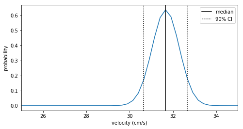
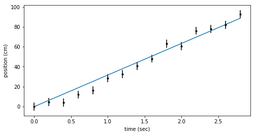
The best fit constant velocity is about \(31.7 \pm 1.0\) cm/s. This looks like it fits the data pretty well.

fig = plt.figure(figsize=(8,4))
ax = fig.add_subplot(111)
ax.errorbar(ts, x_dat, yerr=dx, fmt=".k")
ax.plot(ts, bestfit_line, color='C0')
ax.set_xlabel('time (sec)')
ax.set_ylabel('position (cm)')

constant acceleration (quadratic) model

For the constant acceleration model \(x_0 = 0\), so there are only two free parameters, \(v\) and \(a\).

The Bayesian evidence for the constant acceleration model comes from marginalizing the likelihood over both \(v\) and \(a\). We want the probability for the constant acceleration model averaged over all possible values of \(v\) and \(a\).

\[p\left(d \mid \mathcal{H}_a \right) = \int \mathrm{d}v\,\mathrm{d}a \, p\left(v \mid \mathcal{H}_a \right)\, p\left(a \mid \mathcal{H}_a \right)\, p\left( d \mid \mathcal{H}_a, v, a \right)\]

We use the same Gaussian likelihood, but change our model, \(m\).

\begin{align*} m_i = x_i &= v\, t_i + \frac{1}{2} a\, {t_i}^2, \\
p\left(d \mid \mathcal{H}_v, v \right) &= \left(\frac{1}{\sqrt{2\pi}\,\sigma}\right)^N \exp\left(- \frac{(d_i-m_i)^2}{2{\sigma}^2}\right) \end{align*}

Now we choose our priors, and just like before we will assume ignorance priors. We will keep the same prior for the velocity, \(v \in [0,50]\). For acceleration we will pick \(a \in [-5,15]\).

\[p\left(v \mid \mathcal{H}_a \right) = \frac{1}{\Delta v} = \frac{1}{50}, \quad\quad p\left(a \mid \mathcal{H}_a \right) = \frac{1}{\Delta a} = \frac{1}{20}\]

def prob_quad(params, dat):
    """posterior prob(v,a) for quadratic model
    Gaussian likelihood for params
    uniform prior on v [0,50]
    uniform prior on a [-5,15]
    """
    N = len(dat)
    v, a = params
    if v<0 or v>50 or a<-5 or a>15:
        return 0
    else:
        prior = 1/50 * 1/20  # p(v)*p(a)
    
    mod = pos_v_time(ts, x0=0, v0=v, a0=a)
    norm = (np.sqrt(2*np.pi)*dx)**-N
    arg = -0.5*np.sum((dat - mod)**2)/dx**2
    like = norm * np.exp(arg)
        
    return prior * like

Now we are ready to integrate over \(v\) and \(a\) to compute the marginal likelihood. This 2D integral is a bit trickier, but we still don’t need to get fancy. First, we lay out a rectangular grid in \(v\) and \(a\), and compute the probability at each point.

vs = np.linspace(0, 50, 200)
As = np.linspace(-5, 15, 200)

prob_pts = np.zeros((len(vs), len(As)))
for ii, v in enumerate(vs):
    for jj, a in enumerate(As):
        prob_pts[ii,jj] = prob_quad([v,a], x_dat)

Now we use scipy’s 1D Simpson’s integrator to integrate in each variable one after the other.

int_a = scipy.integrate.simps(prob_pts, x=As, axis=0)
int_v = scipy.integrate.simps(int_a, x=vs)
pquad = int_v
print(pquad)

9.997731977662011e-21

pquad is the Bayesian evidence for the constant velocity model. We’ll come back to the evidences in a moment.

To determine the best fit parameters for the acceleration model, we need to work with the 2D posterior probability.

plt.pcolormesh(As, vs, prob_pts, cmap='Blues')
plt.xlabel("acceleration (cm/s$^2$)")
plt.ylabel("velocity (cm/s)")

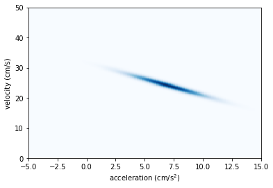
Starting from the full 2D posterior we 1D posteriors for each parameter by marginalizing over the unwanted one. That is we integrate over \(v\) to get the posterior for \(a\) and vice-versa. Then we form the CDF and determine the median values and credible intervals.

apost = scipy.integrate.simps(prob_pts, x=As, axis=0)
vpost = scipy.integrate.simps(prob_pts, x=vs, axis=1)

a_cdf = np.cumsum(apost) / np.sum(apost)  # normalize
v_cdf = np.cumsum(vpost) / np.sum(vpost)

idx_a = a_cdf.searchsorted([0.5, 0.05, 0.95])
idx_v = v_cdf.searchsorted([0.5, 0.05, 0.95])

a_med, a_5, a_95 = As[idx_a]
v_med, v_5, v_95 = vs[idx_v]
print("accel: median = {0:.2f},  90% CI = ({1:.2f} - {2:.2f})".format(a_med, a_5, a_95))
print("vel: median = {0:.2f},  90% CI = ({1:.2f} - {2:.2f})".format(v_med, v_5, v_95))

bestfit_quad = pos_v_time(ts, x0=0, v0=v_med, a0=a_med)

accel: median = 6.96,  90% CI = (3.34 - 10.68)
vel: median = 24.12,  90% CI = (19.85 - 28.14)

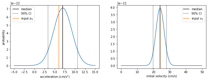
Here we plot the marginalized, 1D posteriors with the medians and 90% confidence intervals marked. We also mark the original values chosen for \(v_0\) and \(a_0\) in the simulation.

fig = plt.figure(figsize=(12,4))
ax1 = fig.add_subplot(121)
ax1.plot(As, apost)
ax1.set_xlabel("acceleration (cm/s$^2$)")
ax1.axvline(x=a_med, color = 'k', label='median')
ax1.axvline(x=a_5, color = 'k', linestyle=':', label=r'90% CI')
ax1.axvline(x=a_95, color = 'k', linestyle=':')
ax1.axvline(x=a0, color = 'C1', label='input $a_0$')
ax1.set_ylabel('probability')
ax1.legend()

ax2 = fig.add_subplot(122)
ax2.plot(vs, vpost)
ax2.set_xlabel("initial velocity (cm/s)")
ax2.axvline(x=v_med, color = 'k', label='median')
ax2.axvline(x=v_5, color = 'k', linestyle=':', label=r'90% CI')
ax2.axvline(x=v_95, color = 'k', linestyle=':')
ax2.axvline(x=v0, color = 'C1', label='input $v_0$')
ax2.legend()

And here’s the best fit quadratic with our data.

fig = plt.figure(figsize=(8,4))
ax = fig.add_subplot(111)
ax.errorbar(ts, x_dat, yerr=dx, fmt=".k")
ax.plot(ts, bestfit_quad, color='C1')
ax.set_xlabel('time (sec)')
ax.set_ylabel('position (cm)')

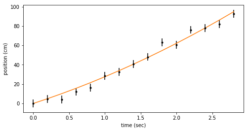
The best fit quadratic also fits these data pretty well. Does it fit better than the line? Are our measurements good enough to say whether or not the particle is accelerating?

Bayes Factor

The Bayes factor is the ratio of the evidences for the two models. If we have no a priori preference for one model over the other, the Bayes factor is equivalent to the betting odds. From the odds we can compute the relative probability for each model.

BF = pquad/pline
prob = 1/(1 + 1/BF)
print("Odds = {0:.0f};  prob = {1:.4f}".format(BF, prob))

Odds = 36;  prob = 0.9733

The quadratic fit is favored over the linear fit at odds 36:1. That works out to a 97% confindence that the particle is accelerating.

Wrap-up

To report our findings we will calculate the difference from the median for each edge of the credible interval.

print(BF, prob)
print(v_med, v_5-v_med, v_95-v_med)
print(a_med, a_5-a_med, a_95-a_med)

36.40104377755644 0.9732627782810682
24.120603015075375 -4.271356783919597 4.0201005025125625
6.959798994974875 -3.618090452261306 3.7185929648241203

We can report that acceleration was favored over constant velocity with a Bayes factor of 36, corresponding to 97% probability. We measured \(v_0 = 24.1^{+4.0}_{-4.3}\) cm/s and \(a_0 = 7.0^{+3.7}_{-3.6}\) cm/s\(^2\), where ranges represent 90% credible intervals. The credible interval in each case contains our original choice for the simulation parameters.

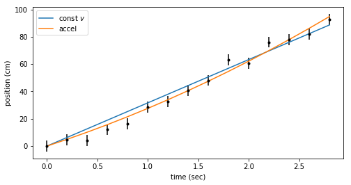
Finally, we show the best fit line and quadratic on the same plot with the data. By eye could you have confidently said one model was better than the other?

fig = plt.figure(figsize=(8,4))
ax = fig.add_subplot(111)
ax.errorbar(ts, x_dat, yerr=dx, fmt=".k")
ax.plot(ts, bestfit_line, color='C0', label='const $v$')
ax.plot(ts, bestfit_quad, color='C1', label='accel')
ax.set_xlabel('time (sec)')
ax.set_ylabel('position (cm)')
ax.legend();

Conclusions

I hope this demostrates that it’s possible use Bayesian data analysis outside of fancy computational methods.