Gravitational Wave Day 2017

Today is the second anniversary of the first direct detection of gravitational waves!

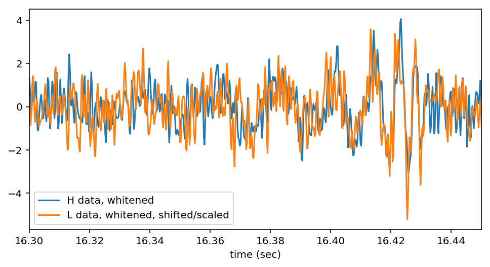
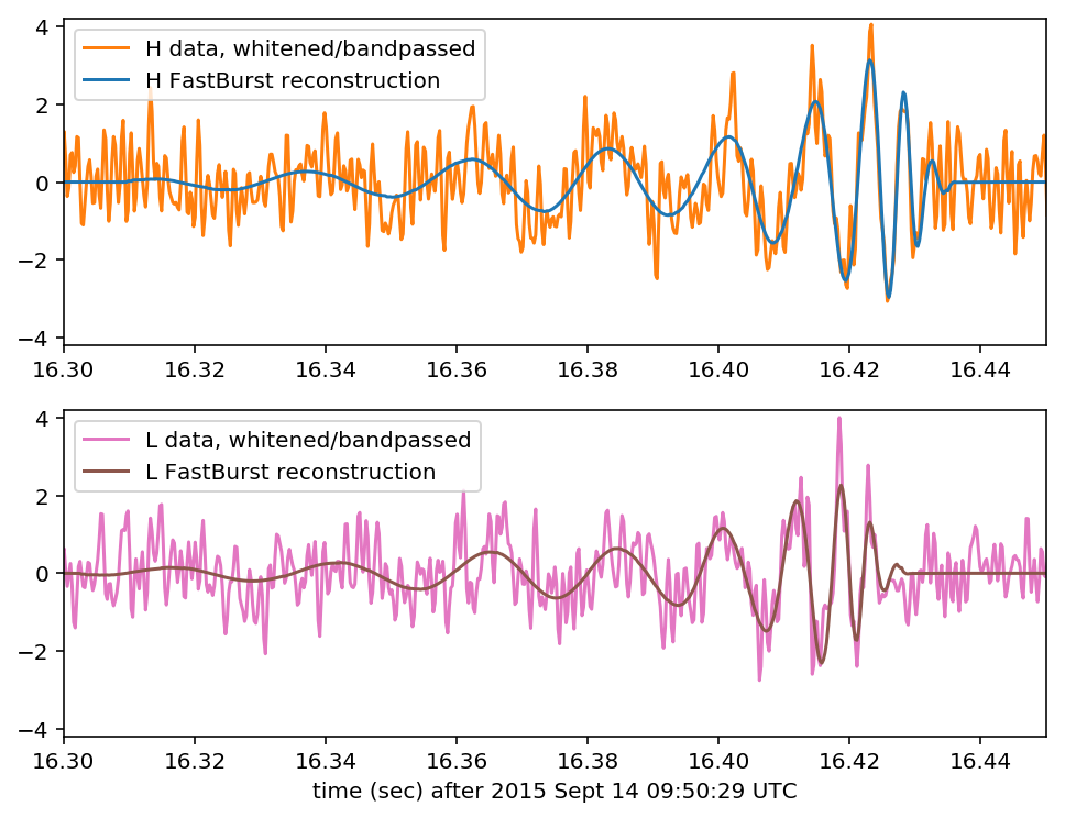
One of the incredible things about the GW150914, the first gravitational wave observed by LIGO, is how loud it was. People like to make a big deal about how you can just see it in the data. In the figure at the top you can “just see” the signal, because the data has been whitened and band-pass filtered. The LIGO noise is frequency dependent or colored. White noise, like white light is the same amplitude at all frequencies. In the figure below you can see the relative amplitude spectral density of the LIGO noise when GW150914 was observed.

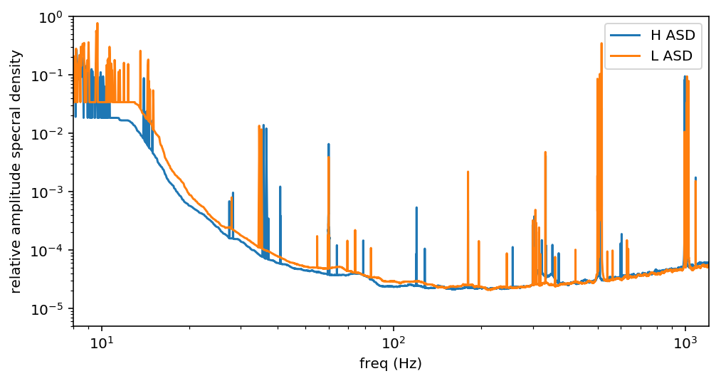
The noise level varies by four orders of magnitude from the low frequencies to where LIGO is most sensitive, around 200 Hz. LIGO is sometimes said to have red noise because the noise is louder at low frequencies, similar to red light. Below we can look at the raw LIGO data from the two detectors side by side. Do you see a gravitational wave?

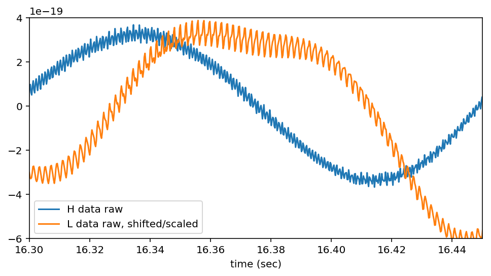
The data shows big slow oscillations with small fast oscillations on top. That’s precisely what red noise looks like. To see the gravitational wave we have to divide out the noise spectrum, down weighting the low frequency data. This also has the effect of setting an amplitude scale.

If the data is just noise, and you divide by the average noise, you should get about 1. If there is loud signal the scaled data should be greater than 1. The whitened data is scaled to the instantaneous signal to noise ratio (SNR).

You can see in the whitened data at the top that the noise bounces around between +1 and -1. If you add up the signal for its whole duration, you would get the total SNR. This is done in practice by integrating the square of the whitened data, which gives the SNR-squared.

Other ways to see GW150914

Another way to “just see” GW150914 in the data is by looking at spectrograms. Spectrograms give information about the amplitude of the signal in both time and frequency. In the spectrograms below you can see the characteristic chirp of a binary merger. The frequency increases with time.

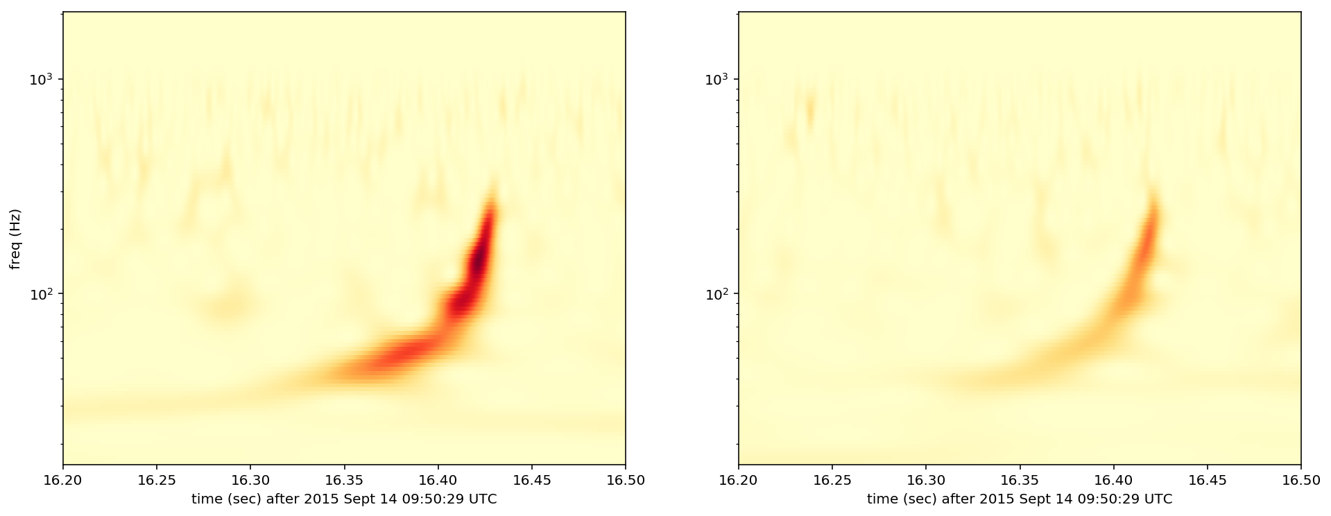
This spectrogram was made by taking a wavelet transform of the data. Spectrograms are a good representation of gravitational wave bursts, that are compact in both time and frequncy That is to say that they are short duration and dominated by a small range of frequencies. In a later post I’ll explain how you can detect bursts of gravitational waves, like GW150914, using wavelets.

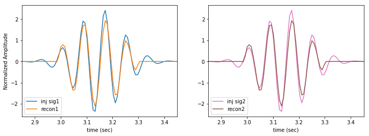
As a teaser, you can oogle a time domain reconstruction of GW150914 using a wavelet denoising algorithm.

LOSC

For this post I used data available from the LIGO Open Science Center (LOSC). The analysis and plots were made in a Jupyter notebook available on my github.