Wavelet Denoising for gravitational wave detection

For this post I’m taking you through a conceptual demonstration of the FastBurst algorithm to find gravitational wave (GW) bursts in LIGO data. This analysis uses no a priori knowledge of GW waveforms.

There are several GW burst searches performed on real LIGO data including Coherent Wave Burst (cWB), BayesWave, and oLIB. This analysis is simple relative to those three, making it a nice introduction to GW burst searching. Do to its simplicity, the FastBurst algorithm is computationally cheap. It is meant to act as a first pass analysis to find times of interest to be analysed by the much more sophisticated and computationally expensive BayesWave pipeline. The production level FastBurst code is written in C, and is being developed for large scale runs on LIGO data.

This first post will go through the basics of wavelet denoising, using a simple simulated gravitational wave signal. In a later post we will see the full process of coherent wavelet denoising, which is the basis of the FastBurst algorithm.

This post was generated from a Jupyter notebook. Did you know you can convert a notebook to markdown?

jupyter nbconvert my_notebook.ipynb --to markdown

I didn’t, but I do now!

If you want to run the notebook yourself, you can get it from my github. This notebook uses my own continuous wavelet transform module, wavelet. It’s not in PyPI yet, but you can install it with pip by following the instructions in the docs

from __future__ import division, print_function, unicode_literals, absolute_import

import numpy as np
import matplotlib.pyplot as plt

import wavelet as w

%matplotlib inline

Generate Data

Wavelet denoising can isolate signals that are compact in both their time and frequency content. So our test signal must have these properties.

We will generate 4 seconds of simulated data sampled at 128 Hz. The data will have a base of white noise with unit variance. To this noise we will inject a gaussian-windowed sinusoidal signal that spans about 1/4 sec of the data. By construction this signal is compact in time (short duration) and in frequency (single dominant oscillation frequency).

\[h(t) = A \exp\left(\frac{-\left(t-t_0\right)^2}{\tau^2}\right)\, \sin\left(2\pi\,f_0\,(t-t_0) + \phi_0\right)\]

\(h(t)\) is defined by five parameters: its amplitude, peak time, damping time, central frequency, and initial phase. Respectively, \((A, t_0, \tau, f_0, \phi_0)\).

LIGO’s detectors also contain non-Gaussian noise artifacts, that look a lot like GW signals. We will also generate a non-Gaussian noise glitch, that is a second gaussian-windowed sinusoid with a different frequency that spans a different (but overlapping) section of the data.

def sine_gaussian(ts, f, amp=1, tau=1, t0=0, phi=0):
    """a gaussian-windowed sinusoid
    h(t) = exp(-(t-t0)^2/tau^2) sin(2*pi*f*(t-t0) + phi)
    """
    win = np.exp(-((ts-t0)/tau)**2)
    sine = np.sin(2*np.pi*f*(ts-t0) + phi)
    return amp*win*sine

Tobs = 4
dT = 1/128
N = int(Tobs/dT)
ts = np.arange(N, dtype=np.float64)*dT
fmax = 1/(2*dT)  # Nyquist frequency (64 Hz)
fmin = 2  # Hz, minimum frequency for plotting.  We could go down to 1/Tobs, but this is fine

# SG 1 -- The Signal
t1 = 3.15  # sec (into data)
f1 = 12 # Hz
tau1 = 1/8 # sec (damp time)
A1 = 2.5
inj = sine_gaussian(ts, f1, A1, tau1, t1)

# SG 2 -- A Glitch
t2 = 3.0  # sec (into data)
f2 = 30  # Hz
tau2 = 0.08 # sec (damp time)
A2 = 3.5
glitch = sine_gaussian(ts, f2, A2, tau2, t2)

# Gaussian Noise
np.random.seed(3333)  # use a defined seed for consistency across runs
noise = np.random.normal(size=N)

# The Total Data
data = noise + inj + glitch

Wavelet transforms are unstable for data with non-zero mean. Lets explicitly set the mean of our data to zero.

data -= data.mean()

Here we plot the simulated data and the injected signal in full and zoomed.

fig = plt.figure(figsize=(16,8))

ax1 = fig.add_subplot(221)
ax1.plot(ts, data, color='C0', label='simulated data')
ax1.set_ylabel("Normalized Amplitude")
ax1.set_xlabel("time (sec)")
ax1.legend(loc='lower left')

ax2 = fig.add_subplot(222)
ax2.plot(ts, data, color='C0')
ax2.set_xlim([2.85, 3.35])
ax2.set_xlabel("time (sec)")

ax3 = fig.add_subplot(223)
ax3.plot(ts, inj, color='C1', label='injected signal')
ax3.plot(ts, glitch, color='C5', label='injected glitch')
ax3.set_ylabel("Normalized Amplitude")
ax3.set_xlabel("time (sec)")
ax3.legend(loc='lower left')

ax4 = fig.add_subplot(224)
ax4.plot(ts, inj, color='C1')
ax4.plot(ts, glitch, color='C5')
ax4.set_xlim([2.85, 3.35])
ax4.set_xlabel("time (sec)")

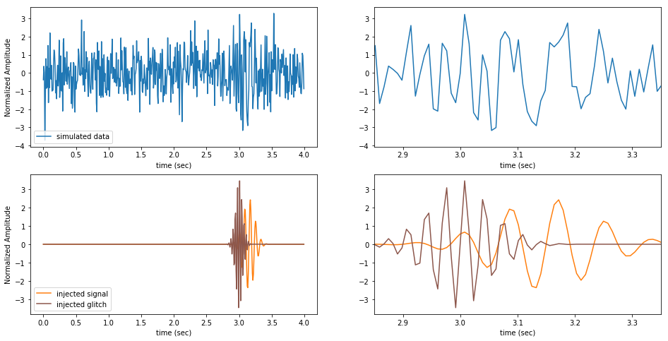
Note how the signal and glitch are individually compact in time, but overlapping.

Single Detector Denoising

As the name indicates, we will be doing our denoising in the wavelet domain.

Wavelet transform

First we need to wavelet transform the data. There are a number of choices to make in the wavelet transform. The provided wavelet module leaves two up to you: the wavelet waveform and the subscale spacing. The subscale spacing sets the frequency resolution of the wavelet transform. It determines the number of frequency scales in each frequency octave. If the subscale spacing is dj = 1/4, then there will be 4 frequency scales between each factor of 2 in frequency.

We will use the Morlet wavelets and set the subscale spacing to dj = 1/16.

First we initialize the WaveletBasis object that sets up the wavelet transform plan for out data specifications. We can read out the frequencies in Hz that correspond to the transform scales. Finally, we perform the continuous wavelet transform and compute the power spectrum.

dJ = 1/16
WB = w.WaveletBasis(wavelet=w.MorletWave(), N=N, dt=dT, dj=dJ)
fs = WB.freqs

wdat = WB.cwt(data)
wpow = np.real(wdat*wdat.conj())

We can take a look at the spectrogram.

fig = plt.figure(figsize=(6,4))
ax = fig.add_subplot(111)
ax.pcolormesh(ts, fs, wpow, cmap='YlOrRd')
ax.set_xlabel("time (sec)")
ax.set_ylabel("freq (Hz)")
ax.set_ylim([fmin, fmax])
ax.set_yscale("log")

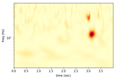
The two big red blobs near 3.0 sec are the injected signal and glitch. In the wavelet domain the two sinusoids separate out into two distinct features. The other high power features come from the random, Gaussian noise.

We will refer to a point in wavelet space defined by at time and frequency as a pixel.

Denoising

To denoise, we simply set a threshold and zero-out any pixels that are smaller than the threshold. This will cut out the noise, while leaving any loud signals intact.

With our unit variance, white, Gaussian noise the pixel amplitude is just to the signal-to-noise ratio (SNR) of that pixel. We can directly set an SNR threshold and use it to denoise the wavelet data array (and power array).

minSNR = 2.0
minPow = minSNR**2

wdat[wpow<minPow] = 0.
wpow[wpow<minPow] = 0.

Now we can take a look at the denoised spectogram.

fig = plt.figure(figsize=(6,4))
ax = fig.add_subplot(111)
ax.pcolormesh(ts, fs, wpow, cmap='YlOrRd')
ax.set_xlabel("time (sec)")
ax.set_ylabel("freq (Hz)")
ax.set_ylim([fmin, fmax])
ax.set_yscale("log")

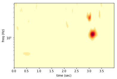
First we see that the signal is preserved, but the glitch also passes the test. The denoising can only eliminate quiet pixels not distinguish signal from non-Gaussian noise. There are also some other places with high power the survive the cut. These arrise from the Gaussian noise. With many samples in our data we should expect the Gaussian noise to fluctuate above the 2-sigma level (i.e. pixel SNR > 2), occationally.

Reconstruction

We can now take the inverse transform of the denoised data to determine the time domain reconstructed signal.

recon = WB.icwt(wdat)

fig = plt.figure(figsize=(12,4))
ax1 = fig.add_subplot(121)
ax1.plot(ts, inj, label='injected signal')
ax1.plot(ts, recon, label='reconstruction')
ax1.set_ylabel("Normalized Amplitude")
ax1.set_xlabel("time (sec)")
ax1.legend(loc='upper left')

ax2 = fig.add_subplot(122)
ax2.plot(ts, inj, label='injected signal')
ax2.plot(ts, recon, label='reconstruction')
ax2.set_xlim([2.85, 3.35])
ax2.set_xlabel("time (sec)")

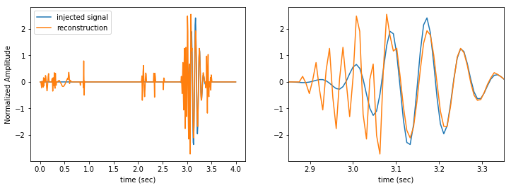
Our reconstructed signal still contains the glitch and a bunch of other noise artifacts. It’s far from perfect, but we can at least tell that there is something in the data.

Coincident Denoising

LIGO uses two detectors to detect GWs. We can leverage the fact that the noise in the detectors should be uncorrelated. If a real GW signal exists in the data, it should appear in both detectors. If a random noise event occurs in one detector, it is very unlikely that a similiar noise event will occur in the other detector.

Simultaneous data

We will regenerate the first data set, with a signal and a glitch. Then we will generate a second data set that contains new, Gaussian noise (with the same statistical properties as before), the exact same signal, but no glitch.

In this case the signals occur simultaneously in each detector at the exact same time. In reality for most GW signals there will be a small temporal offset between the arrival in different detetectors. We will deal with that problem in the next post.

np.random.seed(3333)  # use same random seed to get exact same data!
noise1 = np.random.normal(size=N)
glitch1 = glitch
inj1 = inj
data1 = noise1 + inj1 + glitch1
data1 -= data1.mean()

np.random.seed(7777)  # use different random seed for new noise realization
noise2 = np.random.normal(size=N)
inj2 = inj
data2 = noise2 + inj2
data2 -= data2.mean()

We can wavelet transform these new data using the same WaveletBasis object as the first, because they have the same sampling properties Tobs and dt as the original.

wdat1 = WB.cwt(data1)
wdat2 = WB.cwt(data2)

wpow1 = np.real(wdat1*wdat1.conj())
wpow2 = np.real(wdat2*wdat2.conj())

We can look at the two datasets side by side.

zmax = np.max((wpow1,wpow2))

fig = plt.figure(figsize=(12,4))

ax1 = fig.add_subplot(121)
ax1.pcolormesh(ts, fs, wpow1, cmap='YlOrRd', vmin=0, vmax=zmax)
ax1.set_xlabel("time (sec)")
ax1.set_ylabel("freq (Hz)")
ax1.set_ylim([fmin, fmax])
ax1.set_yscale("log")

ax2 = fig.add_subplot(122)
ax2.pcolormesh(ts, fs, wpow2, cmap='YlOrRd', vmin=0, vmax=zmax)
ax2.set_xlabel("time (sec)")
ax2.set_ylim([fmin, fmax])
ax2.set_yscale("log")

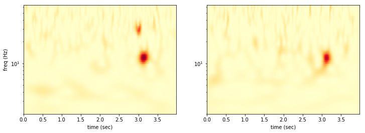
Now we want to find the pixels where the power is above threshold in both detectors simultaneously.

subthresh = np.bitwise_or(wpow1<minPow, wpow2<minPow)  # if *either* is below threshold
wdat1[subthresh] = 0.
wpow1[subthresh] = 0.
wdat2[subthresh] = 0.
wpow2[subthresh] = 0.

fig = plt.figure(figsize=(12,4))

ax1 = fig.add_subplot(121)
ax1.pcolormesh(ts, fs, wpow1, cmap='YlOrRd', vmin=0, vmax=zmax)
ax1.set_xlabel("time (sec)")
ax1.set_ylabel("freq (Hz)")
ax1.set_ylim([fmin, fmax])
ax1.set_yscale("log")

ax2 = fig.add_subplot(122)
ax2.pcolormesh(ts, fs, wpow2, cmap='YlOrRd', vmin=0, vmax=zmax)
ax2.set_xlabel("time (sec)")
ax2.set_ylim([fmin, fmax])
ax2.set_yscale("log")

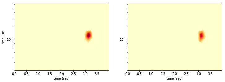
Almost all of the noise is rejected, because the noise is uncorrelated between the detectors. It is very unlikely that the same pixel will have a random 2-sigma fluctuation in both data sets!

The coincident denoising easily rejects the glitch in the first data set!

Now we can inverse wavelet transform and take a look at our reconstructions.

recon1 = WB.icwt(wdat1)
recon2 = WB.icwt(wdat2)

fig = plt.figure(figsize=(12,4))
ax1 = fig.add_subplot(121)
ax1.plot(ts, inj1, color='C0', label='inj sig1')
ax1.plot(ts, recon1, color='C1', label='recon1')
ax1.set_xlim([2.85, 3.45])
ax1.set_ylabel("Normalized Amplitude")
ax1.set_xlabel("time (sec)")
ax1.legend(loc='lower left')

ax2 = fig.add_subplot(122)
ax2.plot(ts, inj2, color='C6', label='inj sig2')
ax2.plot(ts, recon1, color='C5', label='recon2')
ax2.set_xlim([2.85, 3.45])
ax2.set_xlabel("time (sec)")
ax2.legend(loc='lower left')

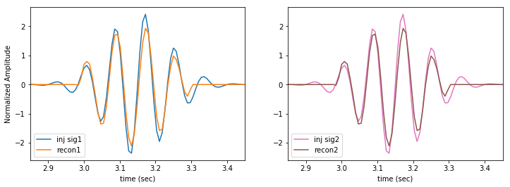
Our reconstruction misses the very quiet tails of the signal, but that should be expected, as we are setting an SNR per pixel threshold. By design we cannot detect quiet features. Unlike a templated search a burst analysis can never detect long, quiet signals. That’s okay. They are not bursts.

More to come

Next time we’ll take a look at how to handle more realistic cases, when there are differences in the time, phase, and amplitude of the signal in each detector.